|
|||||||||||||||||||
|
Trace Analyzer Tool |
|
Johannes Kepler University Altenbergerstr. 69, 4040 Linz, Austria
|
|
|
||
|
Download the Tool
I would be delighted if you find a little bit of time to let me know how you are using this tool and whether or not you find it useful. This page has been viewed
A Mini Tutorial Written by Alexander Egyed DISCLAIMERThis software program and documentation are copyrighted by Alexander Egyed (the author). All Rights Reserved. The software program and documentation are supplied AS IS, without any accompanying services from the author. The author does not warrant that the operation of the program will be uninterrupted or error-free. The end-user understands that the program was developed for research purposes and is advised not to rely exclusively on the program for any reason. IN NO EVENT SHALL THE AUTHOR BE LIABLE TO ANY PARTY FOR DIRECT, INDIRECT, SPECIAL, INCIDENTAL, OR CONSEQUENTIAL DAMAGES, INCLUDING LOST PROFITS, ARISING OUT OF THE USE OF THIS SOFTWARE AND ITS DOCUMENTATION, EVEN IF THE AUTHOR HAS BEEN ADVISED OF THE POSSIBILITY OF SUCH DAMAGE. THE AUTHOR SPECIFICALLY DISCLAIMS ANY WARRANTIES, INCLUDING, BUT NOT LIMITED TO, THE IMPLIED WARRANTIES OF MERCHANTABILITY AND FITNESS FOR A PARTICULAR PURPOSE. THE SOFTWARE PROVIDED HEREUNDER IS ON AN "AS IS" BASIS, AND THE AUTHOR HAS NO OBLIGATIONS TO PROVIDE MAINTENANCE, SUPPORT, UPDATES, ENHANCEMENTS, OR MODIFICATIONS. INTRODUCTIONThe Trace Analyzer is a tool for generating and validating the traceability links among software models, source code, and test scenarios. Models may include any product-relevant model elements such as requirements, architecture, (UML) design, and test scenarios. The Trace Analyzer’s primary task is to reason about the model elements’ ownership of the source code. Its secondary task is to infer trace dependencies among the model elements based on the ownership information. You should use the Trace Analyzer if you have a software system (with or without its source code) with accompanying documentation and models; and you would like to reverse engineer the traceability among the software system, documentation, and models. The tool requires input in form of hypotheses on how the various model elements (requirements, architecture, and design elements) map to the source code. Such hypotheses often exist in legacy documentation; they could also be recovered through testing-and-profiling or brainstorming. It is not expected that such input hypotheses are fully correct and complete. The tool: 1) Refines the input hypotheses by reasoning about their implications and side effects. The resulting knowledge on the model elements’ ownership of the source code is more complete, 2) Indicates conflicts where the input hypotheses are contradictory, 3) Indicates granularity warnings where the input hypotheses are not detailed enough (mutual exclusion problems), 4) Indicates incompleteness, 5) Identifies potential shared code (code that is not owned by a single model element) and utility code (general purpose code that is not owned by any model element although used by it), 6) Generates traceability links among the model elements themselves (among the different diagrams, models, perspectives) based on its refined understanding of the model elements’ ownership of the source code. The tool does not invent traceability information. Such would be silly. Instead, the tool reasons about the given input hypotheses and, in doing so, the tool identifies trace link at different levels of confidence. There are the trace links the tool is confident about. These trace links can be trusted to the degree the input can be trusted. Then there are the trace links the tool believes to be correct. These potential trace links are clearly differentiated from the trusted trace links. The tool cannot guarantee the correctness of any result because this correctness is a function of the correctness of the input hypotheses. However, due to its ability to identify conflicts and granularity issues, the tool’s results are more trustworthy than its input. Moreover, its understanding of the correctness of the trace links is also a function of the completeness of the input. The more complete the input, the more likely a conflict is detected because the space of uncertainty, in which the tool reasons, is smaller. Still, it is possible to get around the tool’s defenses and even a complete input does not guarantee correctness. LAUNCHING THE TOOLClick on the Trace
Analyzer
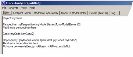
A template set of input hypotheses is provided. Follow its notation. Project: myName Perspective: myPerspective [myModelElement1, myModelElement2] #add more perspectives here Code: [myCode1,myCode2] Dependency: [myModelElement1] isAtMost [myCode1,myCode2] #add more dependencies here #choose between isExactly, isAtLeast, isAtMost, and isNot
The first line is an optional Project name command. Replace myName with an alphanumerical string without spaces. Multiple Perspective lines must follow. A perspective defines a logical grouping of model elements (e.g., the requirements, the state transitions in a statechart diagram) and will be discussed later. A single optional code line may follow that identifies the part of the source code that should be used during the trace analysis. If this line is omitted then all parts of the source code are used. We will talk more about it later. The remaining lines are the actual input hypotheses which are provided with the dependency command. Each input hypothesis defines a mapping between a set of model elements on the left and a set of code elements on the right. Both sets must be enclosed in rectangular brackets ([…]) and if multiple elements are listed, these elements must be separated by a comma (,). The keyword between the two sets defines the nature of the mapping. The choices are isExactly, isAtLeast, isAtMost, isNot, and is. A SMALL EXAMPLEConsider the example of a very simplified Movie Player (Video-On-Demand system). This movie player has: three requirements: Requirement: Stop (not restart) movie at the end Requirement: Start playing movie within 1sec after select Requirement: Allow Image Degradation with low Bandwidth a little statechart diagram (a UML design model):
and a little class diagram (another UML design model):
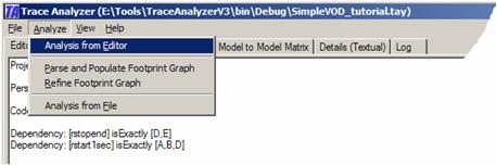
THE REQUIREMENTSOne of the advantages of the Trace Analyzer is that it allows the user to specify the input hypotheses separately for every perspective. As such, the input hypotheses for the requirements can and must be given separately from the input hypotheses for the statechart and class diagram. In the tool, we first define the project name and a perspective for the requirements. Project: SimpleVOD_Tutorial Perspective: r [rstopend, rstart1sec,rdegrade] Names must be unique alphanumerical strings. They may be arbitrarily long but may not contain symbols other than ‘_’. You will see later that short names are better for visualization. The names rstopend, rstart1sec, and rdegrade are short names for the three requirements listed above. We may also define the source code involved. Let us assume that there are six pieces of source code we like to consider. Note that we again use simple short names but these names may also be arbitrarily long alphanumerical string with ‘_’. Code: [A,B,C,D,E,F] These pieces of source code could represent classes, methods, or even lines of code. The tool does not care for as long as you understand what they mean. However, it must be stressed that these pieces of source code must not overlap. It is not allowed that, say, the same method appears in two different pieces. In the following, we refer to pieces of source code as code elements. Without hypotheses on how the requirements map to the source code, the tool cannot do much. The following two input hypotheses define how two of the requirements map to the source code. This input is fairly complete because it defines exactly that rstopend uses D and E – no more, no less; and that rstart1sec uses exactly A, B and D – no more, no less. Dependency: [rstopend] isExactly [D,E] Dependency: [rstart1sec] isExactly [A,B,D] This input is fairly complete because it defines for every requirement separately what it is and what it is not. We will explore less complete input later with the class and statechart diagrams. Now select Analysis from Editor from the Analyze menu to have the tool explore the given input.
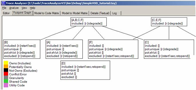
The exact reasoning of the trace analyzer is omitted here. For a detailed description, please read: http://www.alexander-egyed.com/publications/Resolving_Uncertainties_during_Trace_Analysis.pdf However, it is noteworthy that the tool constructs a graph, called the Footprint Graph, visible by clicking on the second tab next to the Editor.
This graph visualizes the tools understanding of the model elements’ ownership of the source code. On the bottom, we have one node per code element. As such, there is a node for code element A and, not surprisingly, the tool believes that this node (i.e., code) is owned by rstart1sec, not owned by rstopend, and potentially own by rdegrade. Note the tool’s separation in what it believes to be correct and what it believes is potentially correct. Also note that there are two potential categories:
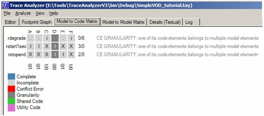
The requirement rdegrade was added to the potentially shared code/utility code category because the tool believes that this code must belong to rstart1sec. However, it would be incorrect to assume that this code cannot also belong to another model element. It is quite possible that a single code element may be owned by multiple model elements (i.e., if it implements different concerns). In fact, if we look at node D (code D) we see that this code belongs to both rstopend and rstart1sec. Thus, while the tool currently believes that code A belongs to rstart1sec, it also thinks it is possible that this code belongs to rdegrate. However, the tool believes that if A also belongs to rdegrade then code A must be shared code or utility code. Note also that nodes C and F list rdegrade under the potential unique category. That is, both nodes are not used by either rstart1sec or rstopend and as such this code could be unique to rdegrade. Finally, note that there are two more nodes above the simple ones. For example, there is a node that groups code elements A, B, C, and F. This node includes the model element rdegrade. What this means is that the tool believes that rdegrade must be inside A, B, C, and/or F but it currently does not know where. Why did the tool single out these four code elements? This has to do with the uniqueness assumption. Every model element inside a perspective must add something unique to the system. Why else would it be there? Thus, there must be some code that is unique to every model elements. We know, from the input, that rstopend must own or share code elements D and E. This statement, triggered by the keyword isExactly, implies that neither rstart1sec nor rdegrade can find their unique code inside D or E (they may find shared code/utility code there but not unique code). Therefore, the tool assumes that both rstart1sec and rdegrade must be with the rest of the code. The tool thus made up another input hypothesis, an implied one: Dependency: [rstart1sec,rdegrade] is [A,B,C,F] The Model to Code Matrix tab summarizes the tools understanding of the model elements’ ownership of the code:
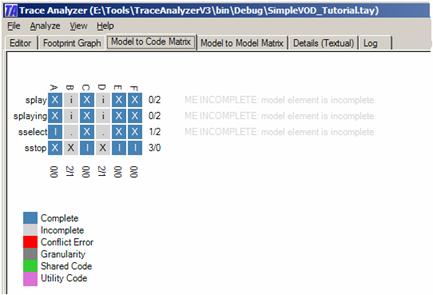
It shows the model elements on the x-axis and the code elements on the y-axis. It says that, say, rstopend owns (I) code E and does not own (X) code B. It also says that rdegrade is not known to own anything but it might potentially own code C as unique code (i) or code B as shared code/utility code (.). The code D is painted in a darker gray because the tool believes it to be either shared code or utility code. The warnings on the right reflect the fact that all three model elements are affected by this knowledge. THE STATECHART DIAGRAMFor simplicity, let us consider the statechart diagram without the knowledge of the requirements. Enter the following information into the editor and select Analysis from Editor from the Analyze menu. Project: SimpleVOD_Tutorial Perspective: s [sselect,splaying,sstop,splay] Code: [A,B,C,D,E,F] Dependency: [sselect,splaying] isAtMost [A,B,D] Dependency: [sstop] isExactly [C,E,F] Dependency: [splay,splaying] isExactly [B,D] This input tells fairly precisely what the sstop transition is about (it owns C, E, and F). However, the remaining input hypotheses are incomplete. We know that both sselect and splaying own at most A, B, and D. This means that sselect owns a subset of A, B, and D – but which subset? We don’t even know whether sselect and splaying own all of A, B, and D. The isAtMost keyword implies this. Similarly, we know that splay and splaying together own all of B and D but we still do not know whether, say, splay owns B or D or both. The tool resolves this to some degree as depicted below.
Although the given input was fairly ambiguous, the tool was able to complete the code elements A, C, E, and F (they are highlighted in blue). But the tool is not quite sure about code elements B and D. More input is required to better understand them. Even though we do not have a complete understanding of the entire code, we actually have some complete understanding of its model elements. We know that model element sstop owns C, E, and F only. It does not own B and D. Model element sstop is not affected by the incompleteness of B and D because it does not own them = thus there is no incompleteness warning for sstop on the right. The other model elements are not complete though. However, we do know that sselect must own code A. This is interesting because this knowledge is not at all obvious from the input. Why does sselect own code A? We know from the input that splay and splaying own code B and D. We also know from the input that sselect must own a subset of A, B, or D. Both statements put together imply that sselect cannot find its unique code in either B or D. Thus, its unique code must be in A. It may still own B or D but in such a case we are certain it would lead to shared code (implied through the ‘.’). THE CLASS DIAGRAMLet’s put all the input hypotheses together and also include hypotheses for the class diagram. Project: SimpleVOD_Tutorial Perspective: r [rstopend, rstart1sec,rdegrade] Perspective: c [cselect,cplay,cstop,cstream,cwait] Perspective: s [sselect,splaying,sstop,splay] Code: [A,B,C,D,E,F] Dependency: [cselect] isAtMost [A,B] Dependency: [cplay,cstream] isExactly [B,D,F] Dependency: [cstop,cwait] isExactly [C,E] Dependency: [cstream] isExactly [D,F] Dependency: [cwait] isExactly [E]
Dependency: [sselect,splaying] isAtMost [A,B,D] Dependency: [sstop] isExactly [C,E,F] Dependency: [splay,splaying] isExactly [B,D]
Dependency: [rstopend] isExactly [D,E] Dependency: [rstart1sec] isExactly [A,B,D]
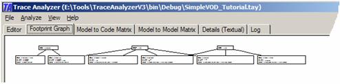
The tool analyzes the different sets input hypotheses for each perspective separately. However, the tool does integrate their results into a single footprint graph.
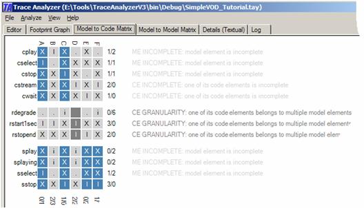
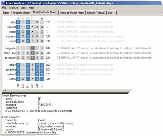
The Model to Code Matrix, however, still visualizes each perspective’s model elements to code mapping separately.
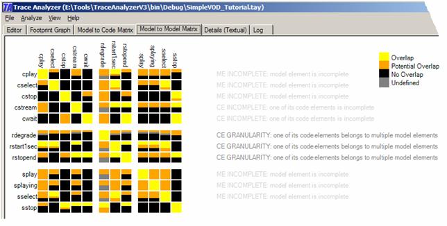
It is important to note that we only have partially complete information at this point. There are several incompleteness warnings across all three perspectives. And there are granularity warnings. We now have two choices: 1) provide more information: this task would be guided by providing more information about those model element and/or code elements that are incomplete. It would not be meaningful to provide more input about model element sstop because it is already complete. Additional input must be added to the editor and then must be re-analyzed. 2) continue with incompleteness Even though the current input in incomplete, we are still able to reason about trace links among the different model elements. Select the Model to Model Matrix tab to visualize the trace links.
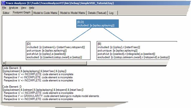
The Model to Model Matrix depicts the same model elements on both axes. It also uses color to indicate whether two model elements have a trace link (yellow), do not have a trace link(black), potentially have a trace link (orange), or are unknown to have a trace link (gray). We see that the state transition sstop has a trace link to rstopend but none to rstart1sec. This implies that the stop transition in the statechart diagram has something to do with the requirement that movies must stop at the end. It also implies that the stop transition has nothing to do with the requirement that movies must start within only 1 second after selecting them. This is fairly intuitive. We also see that the sstop transition has something to do with the cwait method in the class diagram. This is a bit less intuitive. The heavy use of orange in this matrix implies that there is still a lot of uncertainty. For example, the tool believes that there is a potential trace link between splay and cplay. How does the tool compute trace links? The tool does this by looking at any two model elements and reasons about whether their owned code overlap or not. The tool knows that sstop does not own code A, B, and D. The tool also knows that rstart1sec owns this code. Thus both model elements to not share code. If they do not share code, how can they implement a common concern? Note that we distinguish between trace links and uses/calling relationships. This tool does not deal with the latter. The class and statechart diagrams already reveal uses and calling relationships and trace links need to duplicate this. Even through two model elements may use different code, they may end up calling one another and thus affecting one another. However, such calling relationships do not imply similarity among model elements and as such they do not imply trace links. For example, a started movie will eventually stop once it reaches its end. Thus there likely is some calling or data dependency from splay to cstop but this does not mean that splay and cstop are the same. They are not and because of this they are implemented in different code elements. NAVIGATINGThe tool provides a range of powerful navigation and filtering aids. The following describes them. NAVIGATING THE FOOTPRINT GRAPHInside the Footprint Graph, it is possible to select each node through a mouse click. The selected node is highlighted, as are its links to all parent and child nodes. This is useful for navigating the footprint graph. This is also useful for investigating more specific properties about the code elements of the selected node, which are described underneath the graph. For example, the tool writes additional information about the code elements B and D if the node [B,D] is selected. Each code element is listed separately. The first line of each code element lists the different group constraints it must satisfy. As such, code element B must belong to [cplay|cstream] & [splay|splaying] & [rstart1sec] & [cplay]. Also, this code element is incomplete with respect to all perspectives (requirements, statechart, and class).
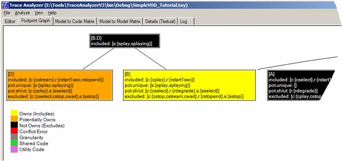
It is possible to highlight individual model elements in the footprint graph by right-clicking on a node. A context menu pops up and it allows you to select any model element listed inside that node. Once selected, the graph changes its coloring to reflect its understanding with respect to the selected model element. Below you see the graph once the model element cplay is selected. It is now easily inferable where that model element in included (yellow), excluded (black), or potentially included (orange).
Furthermore, it is possible to highlight individual perspectives in the footprint graph by right-clicking on the background (an area that is not a node). The graph then visualizes its mapping to all model elements that are part of the same perspective. It is possible to zoom in and out of the graph through the View menu. NAVIGATING THE MODEL TO CODE MATRIXInside the Model to Code Matrix it is possible to select any cell by clicking on it. The tool then visualizes the corresponding model element and code element. For example, the figure below shows what happens if the cwait/E cell is selected. It shows that model element cwait owns code element E and does not own code elements A, B, C, D, and F. Furthermore, it shows that code element E is owned by model element cwait, potentially owned by cstop and not owned by cplay, cselect, and cstream. Note that this output is filtered with respect to the perspective of the selected model element, which is the class diagram in this case. If you like to see another perspective then simply select a cell whose model element belongs to that perspective!
It is also possible to play a limited set of “what happens if” scenarios. Right-click on any cell and you are presented with the context menu that allows you to exclude the selected model element from the cell, declare the code element of this perspective as shared code, or declare the entire code element as utility code. You can undo any of these actions by repeating the same action. Note that these features are somewhat experimental and it is also necessary to invoke Refine Footprint Graph from the Analyze menu to complete this select (this is not done automatically to allow you to make multiple changes at once before refining them). These three features have the following effect:
Note that these features are a non-persistent way of influencing the trace analysis. If you like to make them persistent, you need to add statements to the input hypotheses To exclude a model element from a code element add a dependency: Dependency: [rdegrade] isNot [E] To ignore a code element during the trace analysis, do not list it in the code command. The following input ignores code element F: Code: [A,B,C,D,E] It is not currently possible to make a shared code statement persistent. NAVIGATING THE MODEL TO MODEL MATRIXInside the Model to Model Matrix it is possible to select any cell by clicking on it. Details about the selected model elements are written underneath.
Right-clicking on any cell allows you to change the degree of trustworthiness. You can choose to only visualize overlaps that are known to exist (Display Trace Yes/No). You can also choose to display potential overlaps (Display Trace Yes/Maybe/No). And you can choose to display undefined overlaps (Display Trace Yes/Maybe/Undefined/No). No information is available about undefined overlaps and as such they could be considered potential overlaps – but perhaps with even less confidence about their correctness. The three levels of trust for our sample model are displayed below from left to right.
COPY AND PASTE INTO EXCEL AND OTHER TOOLSThe information depicted in the tool are visually appealing but not readily processable by other tools. Currently the tool does not support import/export mechanisms. However, the Details tab lists much of the graphical information in textual form. It also includes a tab delimitated Model to Model matrix that can be copy-and-pasted to Excel nicely.
DETECTING AND RESOLVING PROBLEMSCONFLICTSOne of the most significant features of the tool is its ability to reason about the correctness of the given input hypotheses. For example, you may notice that it is not possible to simply exclude any model element in the Model To Code Matrix because such an elimination may violate some given input.
For example, if the code element D is excluded from the model element rstopend then the code element turns red. A conflict is detected. This may appear strange because rstopend still has other code elements; or other model elements still use the code element D. Yet, this exclusion contradicts the input that states that rstart1sec is exactly [A,B,D]. Similar conflicts may arise if contradictory input is given. Resolving a conflict requires understanding why it is there. This is not easy at times because the side effects of multiple input hypotheses may have to be considered to understand this reason. Use the navigation features discussed above to learn about the tool’s belief. There are typically two main reasons for conflicts:
Resolve conflicts by changing the input hypotheses. If it is not possible to determine the cause of a conflict, try commenting out input hypotheses to determine which ones are involved. An input dependency can be commented out by placing the pound symbol (#) in front of it: #Dependency: [rdegrade] isNot [E] GRANULARITY WARNINGSA granularity warning is given if there is a model element for which no unique code exists; or if a code element exists that is owned by more than one model elements. A granularity warning may have the following reasons:
A granularity warning does not necessarily imply an error but it should be looked at. INCOMPLETENESSA code element is incomplete if not all model elements are known to own/not own it. A model element is incomplete if it owns a code element that is incomplete. Incompleteness is resolved by adding more input hypotheses. An incompleteness warning does not imply an error. NEED MORE INFORMATION?Please visit http://www.alexander-egyed.com/tools/trace_analyzer_tool.html for up to date information. The Trace Analyzer is a fairly complex piece of logic. It is described in details over a range of publications. The following lists some relevant ones. The first publication provides the most detailed insight into its logic. 1. Egyed, A.: "Resolving Uncertainties during Trace Analysis," Proceedings of the 12th ACM SIGSOFT Symposium on Foundations of Software Engineering (FSE), Newport Beach, California, November 2004, pp.3-12. 2. Egyed A.: A Scenario-Driven Approach to Trace Dependency Analysis. IEEE Transactions on Software Engineering (TSE) 29(2), 2003, 116-132. 3. Egyed, A.: "Tailoring Software Traceability to Value-Based Needs," Book Chapter in Value-Based Software Engineering, Springer Verlag, 2005. 4. Egyed, A. and Grünbacher, P.: "Automating Requirements Traceability - Beyond the Record and Replay Paradigm," Proceedings of the 17th International Conference on Automated Software Engineering (ASE), Edinburgh, Scottland, UK, September 2002, pp. 163-171. 5. Egyed A. and Grünbacher P.: Identifying Requirements Conflicts and Cooperation: How Quality Attributes and Automated Traceability Can Help. IEEE Software 21(6), 2004, 50-58. 6. Egyed, A.: "A Scenario-Driven Approach to Traceability," Proceedings of the 23rd International Conference on Software Engineering (ICSE), Toronto, Canada, May 2001, pp.123-132. CONTACT MEPlease contact me if you have questions. I would like to know how this software is being used to improve your software development process. If you encounter bugs or have recommendations, please let me know. Alexander Egyed (aegyed at ieee.org)
|
||
|
|
||